Measuring Performance¶

Here’s some examples of how to find the optimal worker count and chunk size for different Dask operations. See the scripts in the github repository for samples of how these were measured.

Note

The first time a file is read can be quite slow if it’s not in cache. When running benchmarks make sure to load the file fully once (e.g. with data.mean().load()) before doing any timing.

import pandas
import numpy
import dask
import matplotlib.pyplot as plt

ERA5 single level one year mean¶

Lets look at performance for reading in a year of ERA5 single level data. This data comes from compressed netcdf files, so the time spent decompressing will affect our measurements.

I’ve run for various chunk sizes and Dask cluster sizes

path = "/g/data/rt52/era5/single-levels/reanalysis/2t/2001/2t_era5_oper_sfc_*.nc"
with xarray.open_mfdataset(
    path, combine="nested", concat_dim="time", chunks=chunks
) as ds:
    var = ds[variable]

    start = time.perf_counter()
    mean = var.mean().load()
    duration = time.perf_counter() - start

and saved the results in a netcdf file

df = pandas.read_csv('read_speed/era5_t2_load.csv')
df

	duration	data_size	chunk_size	time	latitude	longitude	workers	threads
0	38.058817	36379929600	194987520	NaN	182	360	4	1
1	38.475415	36379929600	97493760	NaN	182	180	4	1
2	38.962101	36379929600	48746880	NaN	91	180	4	1
3	39.011292	36379929600	97493760	NaN	91	360	4	1
4	50.406360	36379929600	6093360	93.0	91	180	4	1
...	...	...	...	...	...	...	...	...
112	17.296662	36379929600	6093360	93.0	91	180	16	1
113	18.460571	36379929600	97493760	NaN	182	180	16	1
114	18.579301	36379929600	97493760	NaN	91	360	16	1
115	20.263248	36379929600	194987520	NaN	182	360	16	1
116	20.702859	36379929600	389975040	NaN	182	720	16	1

117 rows × 8 columns

To start off with, let’s look at the mean walltime for a given cluster and chunk size. I’ll focus on a single thread as well.

mean = df.groupby(['workers','chunk_size','threads']).mean().reset_index()
one_thread = mean[mean.threads == 1]

and to narrow the results down further I’ll select a single chunk layout of {'time': None, 'latitude': 91, 'longitude': 180}. This is the file chunk size in the horizontal dimensions, about 49 MB per chunk.

df_91_180 = one_thread[(one_thread.latitude==91) & (one_thread.longitude==180) & numpy.isnan(one_thread.time)]
df_91_180 = df_91_180.set_index('workers', drop=False)
df_91_180

	workers	chunk_size	threads	duration	data_size	time	latitude	longitude
workers
1	1	48746880	1	192.943019	3.637993e+10	NaN	91.0	180.0
2	2	48746880	1	86.172158	3.637993e+10	NaN	91.0	180.0
4	4	48746880	1	39.269419	3.637993e+10	NaN	91.0	180.0
8	8	48746880	1	21.874852	3.637993e+10	NaN	91.0	180.0
16	16	48746880	1	13.159739	3.637993e+10	NaN	91.0	180.0
32	32	48746880	1	7.959964	3.637993e+10	NaN	91.0	180.0
48	48	48746880	1	6.344361	3.637993e+10	NaN	91.0	180.0

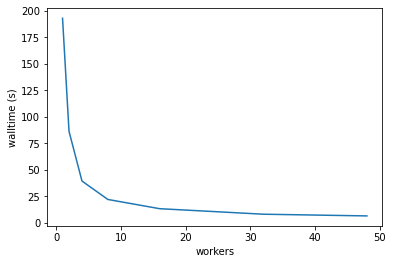
Plotting the walltime taken for different worker sizes looks good, ideally this should be proportional to \( 1 / \textrm{workers}\).

Note

The maximum number of CPUs on a single Gadi node is 48, and the default Dask cluster can’t go beyond that.

wall = (df_91_180['duration'])
wall.plot()
plt.ylabel('walltime (s)');

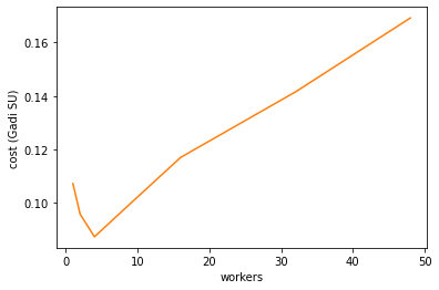
Gadi’s run costs are proportional to \(\textrm{walltime}\times\textrm{workers}\). The cost minimum is at about 4 workers.

Note

Remember this is the cost for just loading the data and calculating the global mean. Further processing can affect the cost scaling as well

cost = (df_91_180['duration'] * df_91_180['workers']/60/60*2)
cost.plot(color='tab:orange')
plt.ylabel('cost (Gadi SU)');

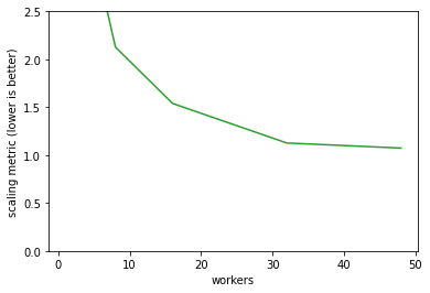
To find a good balance of walltime and cost we want to minimise \(\textrm{walltime}\times\textrm{cost}\). The best worker count by this metric for this single operation is 32 workers.

(wall * cost).plot(color='tab:green')
plt.ylim([0,2.5])
plt.ylabel('scaling metric (lower is better)');

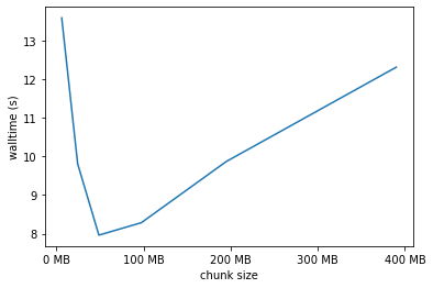
We’ve worked out the best worker count to use, how about the chunk size? The best size here is in the 50 to 100 MB range. Generally the chunk size should be an integer multiple of the file chunk size to make things easy for the NetCDF library, but this doesn’t have a huge effect.

one_thread[one_thread.workers == 32].plot('chunk_size','duration', legend=False)

xlabels = ['0 MB', '100 MB', '200 MB', '300 MB', '400 MB']
plt.xticks([dask.utils.parse_bytes(x) for x in xlabels], labels=xlabels)

plt.xlabel('chunk size');
plt.ylabel('walltime (s)');

def result_scaling(df):
    wall = df['duration']
    cost = df['duration'] * df['workers'] / 60 / 60 * 2
    scaling = wall * cost
    return wall, cost, scaling

def plot_results(csv, target_workers=32):
    df = pandas.read_csv(csv)
    
    mean = df.groupby(['workers','chunk_size','threads']).mean().reset_index()
    one_thread = mean[mean.threads == 1]
    df_91_180 = one_thread[(one_thread.latitude==91) & (one_thread.longitude==180)]
    df_91_180 = df_91_180.set_index('workers', drop=False)
    
    wall, cost, scaling = result_scaling(df_91_180)
    
    ax = plt.subplot(2,3,1)
    wall.plot(ax=ax, color='tab:blue')
    plt.ylabel('walltime (s)');
        
    ax = plt.subplot(2,3,2)
    cost.plot(color='tab:orange')
    plt.ylabel('cost (Gadi SU)');
    
    ax = plt.subplot(2,3,3)
    scaling.plot(color='tab:green')
    #plt.ylim([0,1200])
    plt.ylabel('scaling metric (lower is better)');
    
    df_chunksize = one_thread[one_thread.workers == target_workers].set_index('chunk_size', drop=False)
    wall, cost, scaling = result_scaling(df_chunksize)
    
    xlabels = ['0 MB', '100 MB', '200 MB', '300 MB']
    
    ax = plt.subplot(2,3,4)
    wall.plot(ax=ax, color='tab:blue')
    plt.xticks([dask.utils.parse_bytes(x) for x in xlabels], labels=xlabels)
    plt.xlabel('chunk size');
    plt.ylabel('walltime (s)');
    
    ax = plt.subplot(2,3,5)
    cost.plot(ax=ax, color='tab:orange')
    plt.xticks([dask.utils.parse_bytes(x) for x in xlabels], labels=xlabels)
    plt.xlabel('chunk size');
    plt.ylabel('cost (Gadi SU)');
    
    ax = plt.subplot(2,3,6)
    scaling.plot(ax=ax, color='tab:green')
    plt.xticks([dask.utils.parse_bytes(x) for x in xlabels], labels=xlabels)
    plt.xlabel('chunk size');
    plt.ylabel('scaling metric (lower is better)');

def optimal_size(csv):
    df = pandas.read_csv(csv)
    mean = df.groupby(['workers','chunk_size','threads']).mean().reset_index()
    
    cost = mean['duration']*mean['duration']*mean['workers']
    opt = mean.iloc[cost.sort_values().index[0]]
    print(f'Workers:  {opt.workers:2.0f}')
    print(f'Threads:  {opt.threads:2.0f}')
    print(f"Walltime:  {pandas.Timedelta(opt.duration, 's').round('s')}")
    print(f"Cost:     {(opt.duration/60/60)**2*opt.workers*2:5.2f} SU")
    print(f"Chunks:   {opt[['latitude', 'longitude']].to_dict()}")

ERA5 10-year climatology¶

Calculating a daily mean climatology from 10 years of hourly ERA5 data, using climtas functions for resampling and groupby, saving the results to a compressed netcdf file.

path = "/g/data/rt52/era5/single-levels/reanalysis/2t/200*/2t_era5_oper_sfc_*.nc"
var = 't2m'

with xarray.open_mfdataset(
    path, combine="nested", concat_dim="time", chunks=chunks
) as ds:
    var = ds[variable]
    if isel is not None:
        var = var.isel(**isel)

    out = os.path.join(os.environ['TMPDIR'],'sample.nc')

    start = time.perf_counter()
    daily = climtas.blocked_resample(var, time=24).mean()
    climatology = climtas.blocked_groupby(daily, time='dayofyear').mean()
    climtas.io.to_netcdf_throttled(climatology, out)
    duration = time.perf_counter() - start

plt.figure(figsize=(20,10))
plot_results('read_speed/era5_t2_climatology.csv', target_workers=32)

Workers: 48.0

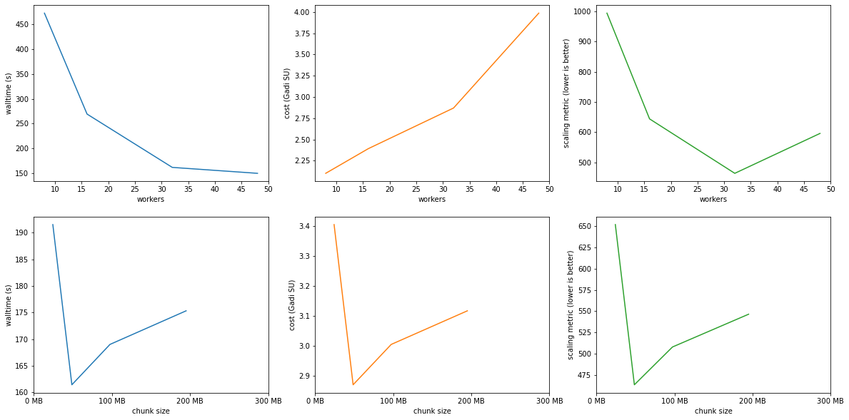
Optimal results:¶

optimal_size('read_speed/era5_t2_climatology.csv')

Workers:  32
Threads:   1
Walltime:  0 days 00:02:41
Cost:      0.13 SU
Chunks:   {'latitude': 91.0, 'longitude': 180.0}

Parallel Programming in Climate and Weather

Measuring Performance¶

ERA5 single level one year mean¶

ERA5 10-year climatology¶

Optimal results:¶